Case Study: Working With Afrobarometer surveys
Source:vignettes/afrobarometer.Rmd
afrobarometer.RmdThe goal of this case study is to explore the variation in trust in various state institutions among African societies, as well as changes in trust over time.
To do this, we use data from Afrobarometer, a cross-national survey project measuring attitudes and opinions about democracy, the economy and society in African countries based on general population samples. Currently, seven rounds of the Afrobarometer are available, covering the period between 1999 and 2019.
retroharmonize is not affiliated with Afrobarometer. To
fully reproduce this example, you must acquire the data files from them,
which is free of charge. Afrobarometer data is protected by copyright.
Authors of any published work based on Afrobarometer data or papers are
required to acknowledge the source, including, where applicable,
citations to data sets posted on this website. Please acknowledge the
copyright holders in all publications resulting from its use by means of
bibliographic citation in this form:
In this vignette, we harmonize data from rounds Afrobarometer Data Round 5 (all countries), Afrobarometer Data Round 6 (all countries) and Afrobarometer Data Round 7 (all countries). Some elements of the vignette are not “live”, because we want to avoid re-publishing the original microdata files from Afrobarometer, but you can access the data directly from the www.afrobarometer.org website.
File names (to identify file versions):
Round 5:
merged-round-5-data-34-countries-2011-2013-last-update-july-2015.sav
Round 6: merged_r6_data_2016_36countries2.sav
Round 7: r7_merged_data_34ctry.release.sav
For reproducibility, we are storing only a small subsample from the
files and the metadata. We assume that you extracted and copied all
.sav files into a single folder that we will call in this
vignette the afrobarometer_dir. Define your
afrobarometer_dir with file.path() in your own
system.
Importing Afrobarometer Files
We start by reading in the three rounds of the Afrobarometer.
### use here your own directory
ab <- dir(afrobarometer_dir, pattern = "sav$")
afrobarometer_rounds <- file.path(afrobarometer_dir, ab)

ab_waves <- read_surveys(afrobarometer_rounds, .f = "read_spss")
Let’s give a bit more meaningful identifiers than the file names:
attr(ab_waves[[1]], "id") <- "Afrobarometer_R5"
attr(ab_waves[[2]], "id") <- "Afrobarometer_R6"
attr(ab_waves[[3]], "id") <- "Afrobarometer_R7"
We can review if the main descriptive metadata is correctly present
with document_surveys().
documented_ab_waves <- document_surveys(ab_waves)
print(documented_ab_waves)
#> # A tibble: 3 × 5
#>   id               filename                               ncol  nrow object_size
#>   <chr>            <chr>                                 <int> <int>       <dbl>
#> 1 Afrobarometer_R5 merged-round-5-data-34-countries-201…   349 51587   159027592
#> 2 Afrobarometer_R6 merged_r6_data_2016_36countries2.sav    365 53935   172064576
#> 3 Afrobarometer_R7 r7_merged_data_34ctry.release.sav       367 45823   148759488
Create a metadata table, or a data map, that contains information
about the variable names and labels, and where each row correspnds to
one variable in the survey data file. We do this with the function
metadata_survey_create(), which extracts the metadata from
the survery data files, normalizes variable labels, identifies ranges of
substantive responses and missing value codes. Its wrapper,
metadata_create(), loops the function on a list of surveys,
or on a set of files containing surveys.
ab_metadata <- metadata_create(survey_list = ab_waves)Working with metadata
From the metadata file we select only those rows that correspond to
the variables that we’re interested in: the rowid being the
unique case identifier, DATEINTR with the interview date,
COUNTRY containing information about the country where the
interview was conducted, REGION with the region
(sub-national unit) where the interview was conducted, and
withinwt being the weighting factor.
Further, we select all variables that have the word “trust” in the normalized variable label.
For these variables, we create normalized variable names
(var_name) and labels (var_label).
library(dplyr)
to_harmonize <- ab_metadata %>%
  filter(var_name_orig %in%
    c("rowid", "DATEINTR", "COUNTRY", "REGION", "withinwt") |
    grepl("trust ", label_orig)) %>%
  mutate(var_label = var_label_normalize(label_orig)) %>%
  mutate(var_label = case_when(
    grepl("^unique identifier", var_label) ~ "unique_id",
    TRUE ~ var_label
  )) %>%
  mutate(var_name = val_label_normalize(var_label))
To further reduce the size of the analysis, we only choose a few
variables based on the normalized variable names
(var_name).
to_harmonize <- to_harmonize %>%
  filter(
    grepl("president|parliament|religious|traditional|unique_id|weight|country|date_of_int", var_name)
  )
The resulting table with information about the variables selected for harmonization looks as follows:
head(to_harmonize %>%
  select(all_of(c("id", "var_name", "var_label"))), 10)
#>                  id                                             var_name
#> 1  Afrobarometer_R5                                            unique_id
#> 2  Afrobarometer_R5                                              country
#> 3  Afrobarometer_R5                                    date_of_interview
#> 4  Afrobarometer_R5 trust_key_leadership_figure_president_prime_minister
#> 5  Afrobarometer_R5                   trust_parliament_national_assembly
#> 6  Afrobarometer_R5                      within_country_weighting_factor
#> 7  Afrobarometer_R6                                            unique_id
#> 8  Afrobarometer_R6                                              country
#> 9  Afrobarometer_R6                                    date_of_interview
#> 10 Afrobarometer_R6                                      trust_president
#>                                               var_label
#> 1                                             unique_id
#> 2                                               country
#> 3                                     date of interview
#> 4  trust key leadership figure president prime minister
#> 5                    trust parliament national assembly
#> 6                       within country weighting factor
#> 7                                             unique_id
#> 8                                               country
#> 9                                     date of interview
#> 10                                      trust president
The merge_surveys() function harmonizes the variable
names, the variable labels and survey identifiers and returns a list of
surveys (of class survey().) The parameter
var_harmonization must be a list or a data frame that
contains at least the original file name (filename),
original variable names (var_name_orig), the new variable
names (var_name) and their labels (var_label),
so that the program knows which variables to take from what files and
how to call and label them after transformation.
merged_ab <- merge_surveys(
  survey_list = ab_waves,
  var_harmonization = to_harmonize
)

# country will be a character variable, and doesn't need a label
merged_ab <- lapply(merged_ab,
  FUN = function(x) {
    x %>%
      mutate(country = as_character(country))
  }
)
Review the most important metadata with
document_surveys():
documenteded_merged_ab <- document_surveys(merged_ab)
print(documenteded_merged_ab)
#> # A tibble: 3 × 5
#>   id               filename                               ncol  nrow object_size
#>   <chr>            <chr>                                 <int> <int>       <dbl>
#> 1 Afrobarometer_R5 merged-round-5-data-34-countries-201…     6 51587    11570496
#> 2 Afrobarometer_R6 merged_r6_data_2016_36countries2.sav      8 53935     8652392
#> 3 Afrobarometer_R7 r7_merged_data_34ctry.release.sav         8 45823     7353968
Harmonization
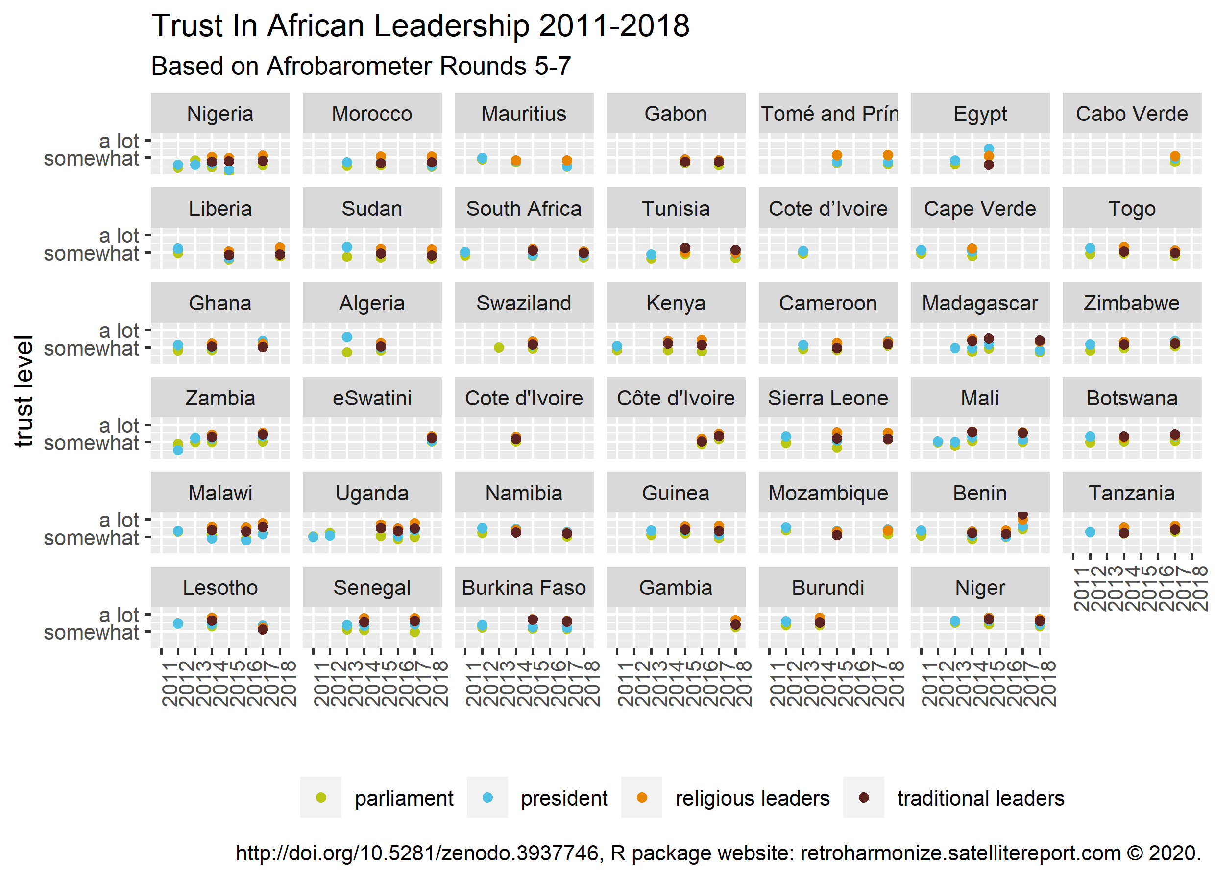
In the Afrobarometer trust is measured with four-point ordinal rating scales. Such data are best analyzed with ordinal models, which do not assume that the points are equidistant. However, to get a quick idea of how the data look like, we will assign numbers 0-3, with 0 corresponding to the least trust, and 3 corresponding to the most trust, and for the time-being analyze the data as if they were metric.
To review the harmonization on a single survey use
pull_survey(). Here we select Afrobarometer Round 6.
R6 <- pull_survey(merged_ab, id = "Afrobarometer_R6")
attributes(R6$trust_president[1:20])
#> $labels
#>                          Missing                       Not at all
#>                               -1                                0
#>                    Just a little                         Somewhat
#>                                1                                2
#>                            A lot Don’t know/ Haven't heard enough
#>                                3                                9
#>                          Refused
#>                               98
#>
#> $label
#> [1] "trust president"
#>
#> $Afrobarometer_R6_name
#> [1] "."
#>
#> $Afrobarometer_R6_values
#> -1  0  1  2  3  9 98
#> -1  0  1  2  3  9 98
#>
#> $Afrobarometer_R6_label
#> [1] "Q52a. Trust president"
#>
#> $Afrobarometer_R6_labels
#>                          Missing                       Not at all
#>                               -1                                0
#>                    Just a little                         Somewhat
#>                                1                                2
#>                            A lot Don’t know/ Haven't heard enough
#>                                3                                9
#>                          Refused
#>                               98
#>
#> $id
#> [1] "Afrobarometer_R6"
#>
#> $class
#> [1] "retroharmonize_labelled_spss_survey" "haven_labelled_spss"
#> [3] "haven_labelled"
The document_survey_item() function shows the metadata
of a single variable.
document_survey_item(R6$trust_president)
#> $code_table
#> # A tibble: 7 × 5
#> values Afrobarometer_R6_values labels Afrobarometer_R6_lab…¹ missing
#> <dbl> <dbl> <chr> <chr> <lgl>
#> 1 -1 -1 Missing Missing FALSE
#> 2 0 0 Not at all Not at all FALSE
#> 3 1 1 Just a little Just a little FALSE
#> 4 2 2 Somewhat Somewhat FALSE
#> 5 3 3 A lot A lot FALSE
#> 6 9 9 Don’t know/ Hav… Don’t know/ Haven't h… FALSE
#> 7 98 98 Refused Refused FALSE
#> # ℹ abbreviated name: ¹Afrobarometer_R6_labels
#>
#> $history_var_name
#> name Afrobarometer_R6_name
#> "R6$trust_president" "."
#>
#> $history_var_label
#> label Afrobarometer_R6_label
#> "trust president" "Q52a. Trust president"
#>
#> $history_na_range
#> character(0)
#>
#> $history_id
#> [1] "Afrobarometer_R6"Afrobarometer’s SPSS files do not mark the missing values, so we have to be careful. The set of labels that are identified as missing:
collect_na_labels(to_harmonize)
#> [1] "Not asked"
The set of valid category labels and missing value labels are as follows:
collect_val_labels(to_harmonize %>%
  filter(grepl("trust", var_name)))
#>  [1] "Missing"                          "Not at all"
#>  [3] "Just a little"                    "Somewhat"
#>  [5] "A lot"                            "Don't know/Haven't heard enough"
#>  [7] "Refused"                          "Don’t know/ Haven't heard enough"
#>  [9] "Don't know/ Haven't heard enough" "Not Asked in this Country"
#> [11] "Not Asked in Country"             "Don’t know/Haven’t heard enough"
#> [13] "Not asked in the country"
We create a harmonization function from the
harmonize_values() prototype function. In fact, this is
just a re-setting the default values of the original function. It makes
future reference in pipelines easier, or it can be used for a question
block only, in this case to variables with
starts_with("trust").
harmonize_ab_trust <- function(x) {
  label_list <- list(
    from = c(
      "^not", "^just", "^somewhat",
      "^a", "^don", "^ref", "^miss", "^not", "^inap"
    ),
    to = c(
      "not_at_all", "little", "somewhat",
      "a_lot", "do_not_know", "declined", "inap", "inap",
      "inap"
    ),
    numeric_values = c(0, 1, 2, 3, 99997, 99998, 99999, 99999, 99999)
  )

  harmonize_values(
    x,
    harmonize_labels = label_list,
    na_values = c(
      "do_not_know" = 99997,
      "declined" = 99998,
      "inap" = 99999
    )
  )
}
We apply this function to the trust variables. The
harmonize_surveys() function binds all variables that are
present in all surveys.
harmonized_ab_waves <- harmonize_surveys(
  survey_list = merged_ab,
  .f = harmonize_ab_trust
)
Let’s look at the attributes of harmonized_ab_waves.
h_ab_structure <- attributes(harmonized_ab_waves)
h_ab_structure$row.names <- NULL # We have over 100K row names
h_ab_structure
#> $names
#> [1] "date_of_interview"
#> [2] "unique_id"
#> [3] "country"
#> [4] "within_country_weighting_factor"
#> [5] "trust_key_leadership_figure_president_prime_minister"
#> [6] "trust_parliament_national_assembly"
#> [7] "trust_president"
#> [8] "trust_traditional_leaders"
#> [9] "trust_religious_leaders"
#>
#> $class
#> [1] "tbl_df"     "tbl"        "data.frame"
#>
#> $id
#> [1] "Waves: Afrobarometer_R5; Afrobarometer_R6; Afrobarometer_R7"
#>
#> $filename
#> [1] "Original files: merged-round-5-data-34-countries-2011-2013-last-update-july-2015.sav; merged_r6_data_2016_36countries2.sav; r7_merged_data_34ctry.release.sav"
Let’s add the year of the interview:
harmonized_ab_waves <- harmonized_ab_waves %>%
  mutate(year = as.integer(substr(as.character(
    date_of_interview
  ), 1, 4)))
To keep our example manageable, we subset the datasets to include only five countries.
Analyzing the harmonized data
The harmonized data can be exported and analyzed in another
statistical program. The labelled survey data is stored in
labelled_spss_survey() vectors, which is a complex class
that retains metadata for reproducibility. Most statistical R packages
do not know it. The data should be presented either as numeric data with
as_numeric() or as categorical with
as_factor(). (See more why you should not fall back on the
more generic as.factor() or as.numeric()
methods in The
labelled_spss_survey class vignette.)
Please note that the numeric form of these trust variables is not directly comparable with the numeric averages of the Eurobarometer trust variables, because the middle of the range is at 1.5 and not 0.5.
harmonized_ab_waves %>%
mutate_at(
vars(starts_with("trust")),
~ as_numeric(.) * within_country_weighting_factor
) %>%
select(-all_of("within_country_weighting_factor")) %>%
group_by(country, year) %>%
summarize_if(is.numeric, mean, na.rm = TRUE)
#> # A tibble: 17 × 7
#> # Groups: country [5]
#> country year trust_key_leadership…¹ trust_parliament_nat…² trust_president
#> <chr> <int> <dbl> <dbl> <dbl>
#> 1 Algeria 2013 2.59 1.70 NaN
#> 2 Algeria 2015 NaN 1.82 2.00
#> 3 Madagasc… 2013 1.96 NaN NaN
#> 4 Madagasc… 2014 NaN 1.75 1.95
#> 5 Madagasc… 2015 NaN 1.94 2.15
#> 6 Madagasc… 2018 NaN 1.71 1.83
#> 7 Niger 2013 2.59 2.52 NaN
#> 8 Niger 2015 NaN 2.43 2.64
#> 9 Niger 2018 NaN 2.31 2.42
#> 10 Nigeria 2012 1.59 1.43 NaN
#> 11 Nigeria 2013 1.59 1.84 NaN
#> 12 Nigeria 2014 NaN 1.45 1.64
#> 13 Nigeria 2015 NaN 1.15 1.30
#> 14 Nigeria 2017 NaN 1.57 2.06
#> 15 South Af… 2011 2.04 1.84 NaN
#> 16 South Af… 2015 NaN 1.82 1.87
#> 17 South Af… 2018 NaN 1.70 1.86
#> # ℹ abbreviated names: ¹trust_key_leadership_figure_president_prime_minister,
#> # ²trust_parliament_national_assembly
#> # ℹ 2 more variables: trust_traditional_leaders <dbl>,
#> # trust_religious_leaders <dbl>And the factor representation, without weighting:
library(tidyr) ## tidyr::pivot_longer()
harmonized_ab_waves %>%
  select(-all_of("within_country_weighting_factor")) %>%
  mutate_if(is.labelled_spss_survey, as_factor) %>%
  pivot_longer(starts_with("trust"),
    names_to  = "institution",
    values_to = "category"
  ) %>%
  mutate(institution = gsub("^trust_", "", institution)) %>%
  group_by(country, year, institution, category) %>%
  summarize(n = n())
#> `summarise()` has regrouped the output.
#> ℹ Summaries were computed grouped by country, year, institution, and category.
#> ℹ Output is grouped by country, year, and institution.
#> ℹ Use `summarise(.groups = "drop_last")` to silence this message.
#> ℹ Use `summarise(.by = c(country, year, institution, category))` for
#>   per-operation grouping (`?dplyr::dplyr_by`) instead.
#> # A tibble: 311 × 5
#> # Groups:   country, year, institution [85]
#>    country  year institution                                    category       n
#>    <chr>   <int> <chr>                                          <fct>      <int>
#>  1 Algeria  2013 key_leadership_figure_president_prime_minister little        75
#>  2 Algeria  2013 key_leadership_figure_president_prime_minister somewhat     341
#>  3 Algeria  2013 key_leadership_figure_president_prime_minister a_lot        759
#>  4 Algeria  2013 key_leadership_figure_president_prime_minister do_not_kn…    13
#>  5 Algeria  2013 key_leadership_figure_president_prime_minister inap          16
#>  6 Algeria  2013 parliament_national_assembly                   little       317
#>  7 Algeria  2013 parliament_national_assembly                   somewhat     419
#>  8 Algeria  2013 parliament_national_assembly                   a_lot         95
#>  9 Algeria  2013 parliament_national_assembly                   do_not_kn…   131
#> 10 Algeria  2013 parliament_national_assembly                   inap         242
#> # ℹ 301 more rows
We subsetted the datasets to meet the vignette size limitations. If you are following our code without reducing the number of countries, you get the following results: